I developed this demonstration in R to teach my students about classical hypothesis testing and p-values.
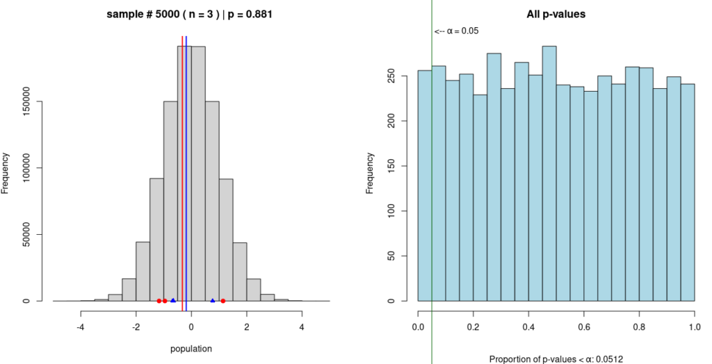
In this Monte Carlo simulation, two random samples are taken from a single, known population; in this case, the population is normally distributed, as can be seen in the grey histogram on the left. One sample is represented by blue dots and the other by red dots, with the mean of each sample represented by a vertical line of the same color.
A t-test is performed on the means of the two samples to compute a p-value. This procedure is repeated 4,999 more times; each time, the new p-value is added to the growing histogram of p-values on the right.
The purpose of this simulation is to demonstrate that p < 0.05 does not prove the alternative hypothesis. In this simulation, the alternative hypothesis is that the two samples come from different populations. And while about 5% of the p-values in the simulation do fall below 0.05, we know for a fact that the alternative hypothesis is false, because the simulated samples are coming from the same population.
The code I used to perform this simulation is below. Note that parameters such as population size, population distribution, sample size, number of times to repeat the simulation, and the alpha level can all be adjusted by modifying the first several lines of code.
### DEMO - Monte Carlo simulation: interpreting a t-test p-value --------------------
# Written by Dr. Taylan Morcol, PhD (https://morcol.com)

N <- 1000000 # population size

population <- rnorm(N) # random sample of the standard normal distribution
hist(population) # visualize the population

NS <- 5000 # number of times to sample
n <- 3 # sample size
a <- 0.05 # alpha level (tolerance for Type I errors)
plot.t <- FALSE # should histogram of t-values be included?

par(mfrow=c(1,if(plot.t){3}else{2})) # 1 x 2 graphics window

p <- c() # empty vector to hold p-values
tvals <- c() # empty vector to hold t-values
for(i in 1:NS){
   s1 <- sample(population, n, replace=TRUE)
   s2 <- sample(population, n, replace=TRUE)

   out <- t.test(x=s1, y=s2, var.equal=TRUE)
   p.i <- out$p.value
   p <- c(p, p.i)
   t.i <- out$statistic
   tvals <- c(tvals, t.i)

   p.title <- paste("sample #", i, "( n =", n, ") | p =", signif(p.i, 3), if(p.i <= a){"*"})
   hist(population, main=p.title) # histogram of population

   points(x=s1, y=rep(0, n), type="p", pch=19, col="red") # sample 1 points
   abline(v=out$estimate[1], lwd=2, col="red") # sample 1 mean

   points(x=s2, y=rep(0, n), type="p", pch=17, col="blue") # sample 2 points
   abline(v=out$estimate[2], lwd=2, col="blue") # sample 2 mean

   prop.p <- sum(p < a)/length(p) # proportion of p-values less than alpha

   hist(p, col="lightblue", breaks=1/a # histogram of all p-values so far
      , xlim=c(0,1), xlab=""
      , main="All p-values"
      , sub=paste("Proportion of p-values < \U03B1:", signif(prop.p,3))
   ) # end hist()

   abline(v=a, col="darkgreen", xpd=TRUE) # line at cutoff for significance
   mtext(paste(" <-- \U03B1", "=", a), side=3, at=a, adj=0) # label for line above

   if(plot.t){hist(tvals, col="peru")} # end hist()

   # slower in beginning (for screen recording); comment out if not recording
   #if(i < 5){Sys.sleep(4)} else if(i < 10){Sys.sleep(2)} else if(i < 15){Sys.sleep(1)}

   #readline(prompt="Press [Enter] to continue...") # comment out if non-interactive

} # end for() loop