
Background and overview
Last year, after finishing grad school, I decided to shift to a career in freelance work.
Being relatively new to freelancing, I decided to take the Endless Freelance Income course, which is designed to guide people transitioning from academia to freelancing. The third chapter of the course is all about choosing a niche. Much of this chapter involves using Upwork to research the freelance job market.
In this article, I’ll walk through the steps I took to evaluate one aspect of the freelance job market: labor market saturation (i.e., competition for jobs). This is important because if there are a lot of other freelancers applying for jobs in a given category, it could be harder to get jobs in that category. And vice versa.
So my goal here is to determine if any job categories I’m interested in have relatively low job competition.
Keep in mind that job competition is only one of several factors that I’m considering, including number of available jobs, income potential, required skills, and my interests.
I chose to write about my job competition research because I saw an opportunity to do some fun data analysis and share it with the world.
Throughout this article, I discuss my reasoning for doing things in certain ways. I also include the R code I used so that those who are interested can follow along.
If you just want to skip ahead to the main results, you can go here, here, and here.
Getting raw data from Upwork.com
The first step was to extract data from Upwork’s job search.
The approximate number of proposals for each job are indicated by one of six predefined ranges: less than 5, 5 to 10, 10 to 15, 15 to 20, 20 to 50, and 50+. This introduces some uncertainty into the analysis. (More on that later.)
For each job category, I looked at the first two pages of jobs–or all jobs if there were less than two pages worth–and I copied the upper end of the proposal number range for each job into a spreadsheet
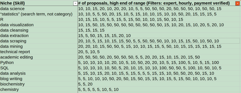
FYI, this list was prescreened to include only job categories that I am interested in, that match my current skills (or skills I want to learn), and that have good income potential (based on hourly pay rates).
Formatting the data for R
Before importing the spreadsheet into R, I made two changes to make the data easier to work with in R.
First, I simplified the column headers:
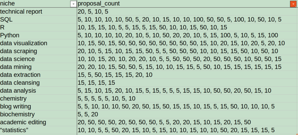
Second, I saved the spreadsheet as a CSV file, which is a simpler format than XLSX or ODS and is easier to import into R.
Data import and wrangling in R
Here’s the R code I used to import and clean up the data:
# initial params/variables
wd <- "/home/tay/Documents/Endless_Freelance_Income_course/Homework/"
td <- "/home/tay/Desktop/Temp/" # temporary directory
data_file_name <- "CH3L1_Worksheet_ResearchingPotentialNiches_20220504.csv"

# data import
setwd(wd)
raw_csv <- read.csv(data_file_name)

# removing extraneous columns and rows
colnames(raw_csv) # to check column names
dfr <- raw_csv[, c("niche", "proposal_count")] # extract relevant columns
dfr <- dfr[which(dfr$proposal_count != ""),] # remove niche categories with no proposal count data
Next, I loop through each job category, parsing the comma-separated job counts data to put each data point in a separate cell:
dfr2 <- c()
for(i in 1:length(dfr$proposal_count)){
    counts <- as.numeric(unlist(strsplit(dfr$proposal_count[i], split=",")))
    temp <- cbind(niche=rep(dfr$niche[i], length(counts)), counts=counts)
    dfr2 <- rbind(dfr2, temp)
} #end for()
At this point, dfr2 is a matrix with all data as the “character” type:
> str(dfr2)
 chr [1:250, 1:2] "technical report" "technical report" "technical report" ...
 - attr(*, "dimnames")=List of 2
  ..$ : NULL
  ..$ : chr [1:2] "niche" "counts"
But I want a dataframe (not a matrix) with data types “factor” (for niche) and “integer” (for counts).
I could use functions to convert dfr2 to a dataframe and change the data type of each of the vectors individually. But I’ve found this way to be cumbersome and non-intuitive.
So instead, I export as a temporary CSV and then re-import that same CSV:
temp_csv_path <- paste(td, "temp.csv", sep="")
write.csv(dfr2, file=temp_csv_path, row.names=FALSE)
dfr2 <- read.csv(temp_csv_path, stringsAsFactors=TRUE)
The read.csv() function formats data in a way that is intuitive for me. Now my data are formatted the way I want:
> str(dfr2)
'data.frame':	250 obs. of  2 variables:
 $ niche : Factor w/ 16 levels "“statistics”",..: 16 16 16 16 15 15 15 15 15 15 ...
 $ counts: int  20 5 10 5 5 10 10 10 10 50 ...
Prep work for making histograms
Because of the uncertainty in the exact number of proposals for each job, I chose to visualize the data using histograms, with bins corresponding to Upwork’s predefined job count ranges. If this doesn’t make sense yet, stick with me.
But before making the histograms, some more data wrangling is in order.
First, I do a some number replacements. In retrospect, I could have done this when I was recording the proposal counts from Upwork. But my thoughts on how to do this analysis evolved over time, so I am replacing the numbers after the fact:
dfr2$counts[which(dfr2$counts == 5)] <- 3
dfr2$counts[which(dfr2$counts == 10)] <- 7
dfr2$counts[which(dfr2$counts == 15)] <- 13
dfr2$counts[which(dfr2$counts == 20)] <- 17
dfr2$counts[which(dfr2$counts == 50)] <- 35
dfr2$counts[which(dfr2$counts == 100)] <- 75
Before making these replacements, the proposal count for each job was represented by the upper end of its range. After replacement, the proposal count for each job is represented by a number somewhere in the middle of its range. In this way, the numbers still uniquely represent the ranges into which they fall.
Next, I sort the niche categories in increasing order of median proposal counts:
dfr2$niche <- with(dfr2, reorder(niche, counts, median, na.rm=TRUE))
Note that replacing the numbers changes the median values themselves but preserves the relative order of the median values.
Next, I define/calculate some parameters that I will later use for making the histogram plots:
n <- length(unique(dfr2$niche)) # number of job categories
brks <- c(0,5,10,15,20,50,100) # breaks defining the histogram "bins", which correspond to Upwork's predefined proposal count ranges

bin_counts <- c()
for(i in 1:n){
    j <- which(dfr2$niche == levels(dfr2$niche)[i])
    tmp <- hist(x=dfr2$counts[j], breaks=brks, plot=FALSE)
    bin_counts <- c(bin_counts, tmp$counts)
} #end for()
y_max <- max(bin_counts) # this variable will be used to plot all histograms on the same y-axis scale
Making histograms in R
Now for the fun part: visualizing the data!
I generate histograms and save as an SVG file:
svg(file="Ch3L1_Histograms_JobCompetition.svg", width=7, height=10)
par(mfrow=c(n,1), mar=c(1,2.5,1,1), oma=c(4,3,0,0))
for(i in 1:n){
    j <- which(dfr2$niche == levels(dfr2$niche)[i])
    N <- length(dfr2$counts[j]) # sample size
    hist(x=dfr2$counts[j], breaks=brks
       , xaxt="n", main=""
       , cex.axis=1.5
       , ylim=c(0,y_max), freq=TRUE)
    med <- median(dfr2$counts[j])
    abline(v=med, col="red")
    label <- paste(levels(dfr2$niche)[i], "  (N=", N, ")",sep="")
    mtext(text=label, side=3, line=-1, cex=1.4, adj=1)
} #end for()
axis(side=1, at=brks, labels=brks, cex.axis=1.5, las=3, xpd=TRUE)
mtext("number of proposals"
    , side=1, line=2.5, cex=1.5, outer=TRUE)
mtext("number of jobs"
    , side=2, line=0.5, cex=1.5, outer=TRUE)
dev.off()
Here’s what the plot looks like:

A word about statistical significance testing
Examining the histograms above, there do appear to be some differences in labor market saturation between freelance job categories.
But are any of these differences statistically significant? Put another way, what are the odds that the observed differences are due to random variation than to actual differences between the groups?
ANOVA is the most commonly used test in this type of situation. But I decided against using ANOVA, mainly because it relies on accurately calculating means. Recall that there is substantial uncertainty about the exact number of proposals per job in each of the predefined job count ranges, which makes it impossible to accurately calculate mean values from the available data. ANOVA also assumes that the data are normally distributed; based on visual inspection of the histograms, this does not seem to be the case.
On the other hand, the Kruskal-Wallis test does not assume normality and is based on ranks of median values, which are less affected by the uncertainty in this dataset.
However, like ANOVA, the Kruskal-Wallis test also assumes that the data points in each category are independent of all other categories. But as I mentioned earlier, the job categories that I defined are not mutually exclusive; there is overlap between categories (e.g., the data science category likely contains job listings that are also tagged as data visualization jobs).
So this dataset violates the assumption of independent observations. While statistical tests can be robust to violations of some assumptions, a violation of the assumption of independent observations is generally more problematic.
Nonetheless, I think that significance testing is still somewhat helpful for understanding trends in these data. Just keep in mind moving forward that the freelance job categories are not completely distinct from one another and that the conclusions we can draw from significance testing are thus limited.
Testing for statistical significance between freelance job categories in R
As I mentioned earlier, the Kruskal-Wallis test compares the ranks of proposal counts rather than the counts themselves. And the relative order of the proposal counts is unchanged by the number replacements I did earlier.
Performing a Kruskal-Wallis test in R is pretty simple:
kruskal.test(counts ~ niche, data=dfr2)
And the results:
> kruskal.test(counts ~ niche, data=dfr2)

	Kruskal-Wallis rank sum test

data:  counts by niche
Kruskal-Wallis chi-squared = 36.278, df = 15, p-value = 0.001611
The p-value is roughly 0.0016, which is less than the 0.05 minimum value typically used to determine statistical significance. Thus, there appears to be a statistically significant difference in labor market saturation between at least two of the job categories.
But which categories?
To address this question, I used Dunn’s test, a non-parametric analog to the Tukey HSD test. I performed this in R with the help of the “dunn.test” package:
library(dunn.test)
dunn_out <- dunn.test(x=dfr2$counts, g=dfr2$niche, method="holm", list=TRUE)
Now some data wrangling to view the results more clearly:
dunn_dfr <- data.frame(P_adj=dunn_out$P.adjusted, comparison=dunn_out$comparisons)
dunn_dfr <- dunn_dfr[order(dunn_dfr$P_adj),]
And the results of Dunn’s test, sorted by adjusted p-value:
> print(dunn_dfr, row.names=FALSE)
        P_adj                            comparison
 0.0008899786          academic editing - chemistry
 0.0009650131        chemistry - data visualization
 0.0044175891              chemistry - data science
 0.0653044907               chemistry - data mining
 0.0803192084             chemistry - data scraping
 0.2964815493                       chemistry - SQL
 0.3728975842           chemistry - data extraction
 0.4007177072             chemistry - data analysis
 0.4579814069              blog writing - chemistry
 0.4995643595                 “statistics” - Python
The results of this test indicate significant differences (p < 0.05) between:
- chemistry and academic editing
- chemistry and data visualization
- chemistry and data science
In all cases, the significant differences are between chemistry and another job category. In fact, the nine lowest p-values are all between chemistry and another category.
These results make sense in combination with the histograms, which show that chemistry has one of the lowest median proposal counts and the lowest maximum number of proposals.
One may then ask why biochemistry, which was tied with chemistry for lowest median proposal counts, doesn’t show up in the list of lowest p values. My guess is that the sample size for biochemistry (N=3) was too low to yield significant p values.
Any clear winners?
The histograms and (flawed) significance testing suggest that the chemistry market may have lower job competition than most other categories in this analysis.
Recall that the main problem with the significance testing was a violation of the assumption of independent observations due to cross-listing between job categories. But from my recollection, there was little cross-listing between chemistry and other categories (except for biochemistry). For this reason, I have more confidence that job competition is significantly less in chemistry.
But again, because the assumption of independent observations was violated, strictly speaking there were no clear significant differences in labor market saturation among the categories analyzed.
Other considerations
In the end, competition for jobs is only one of several considerations in choosing a freelance niche. I am also considering other factors, such as number of available jobs, income potential, required skills, and my own interests.
With that in mind, let’s take another look at the chemistry job category. Assuming for a moment that this category does in fact have less job competition than the others, does this look like a good niche for me?
In a word, no. Here are a few reasons why:
- Small number of opportunities. Taking another look at the histograms, you can see that there were only eight job listings (N=8) in the whole category. And this number likely includes job listings that were posted weeks or even months ago and are not actually available anymore.
- Highly specialized requirements. From my notes, the chemistry jobs generally require highly specialized subject-area expertise–such as product formulation–that I don’t have.
In summary
I started this assignment with a simple question: how does competition for freelance jobs compare across the freelance niches that I am interested in? The analyses reveal some potential differences between the job categories. But the non-independent nature of the data points prohibit any definitive conclusions about the statistical significance of these differences.
So in the end, I’m choosing my freelance niche–data science with a specialty in statistics–based not only on my analysis of job competition but also on other considerations. For one, I love statistics and looking for trends in data (as you may be able to tell). Also, the income potential for these types of jobs looks relatively high (data not shown). And, although the difference is not statistically significant, the histograms still suggest relatively lower job competition in the “statistics” category.
In the future
One thing that could be improved about this analysis is the sample size. Because I was manually scraping data from Upwork.com, I only sampled the first two pages of job listings (up to 21 listings) per category. In some cases, this sample represented only a small fraction of the jobs listed for a category. In the future, I could use an API like this one to gather more data faster, which would give me a more representative picture of competition in the freelance job market.
Another thing to consider is that job competition could depend, in part, on income potential. In other words, a particular niche could have higher competition because it has higher paying jobs. A regression analysis could be used to investigate the influence of pay rate on job competition.
Last but not least, how to address the issue of cross-listing among categories? One way could be to select job categories that are largely exclusive of one another and/or eliminate any cross-listed jobs. However, I have a hunch that doing so would eliminate a lot of valuable data and limit the categories that I can compare. So perhaps using a statistical framework that does not assume independent observations would be better suited.
All of these options sound pretty interesting to me. Perhaps I’ll explore them in another article… 🤔
RESOURCES
- Endless Freelance Income, an online course designed to guide people from academia into freelance work
- Upwork.com, one of the largest freelance job listing platforms
- R, a programing language that is well-suited for doing statistical analyses
- dunn.test, an R package for performing Dunn’s test
Did you learn something new? How would you have done this analysis differently?
I’d love to hear your thoughts in the comments below. Please teach me something!
This is so fascinating! Thanks for sharing your process.