
This is the third in a series of articles looking at plant diversity in my small, home garden. The first one presented the results of a botanical inventory I did about a month ago, which included total and proportional cover for each plant species.
The second one compared those results to an inventory–reconstructed from memory–of the same area of land before I started gardening. I used this comparison to explore the concepts of species richness (i.e., the total number of species) and evenness (i.e., how closely the relative abundances match among species). Both richness and evenness are aspects of diversity.
It was clear just from looking at the raw species cover data that richness had increased as a result of my gardening activities. Richness is a fairly straightforward measure of diversity, but it’s crude because it does not take evenness into account. I ended that article saying I’d next explore more complex measures of diversity that take into account both richness and evenness. This is what I will write about in the current article.
A few words about indices
The past two weeks, I have been learning about species diversity indices. I found a 2021 Oikos paper by Roswell and colleagues that helped me understand the why’s and how’s of some common indices. This paper explains the relatively new concept of Hill diversity–a general approach to calculating diversity–and compares three special cases of Hill diversity with their traditional counterparts: species richness, Shannon index, and Simpson index. The authors argue that the Hill versions of Shannon and Simpson indices are more intuitive in their interpretations than their traditional counterparts, while Hill richness and traditional richness are one and the same metric. To illustrate these points, I am going to show the species cover data from the two inventories along with calculated values of each of the five diversity indices.
A bit of context. From what I understand, traditional diversity indices were developed to use individual counts as a measure of species abundance. But as I mentioned in my first article, I chose to measure species abundance in terms of area cover. I did this because for many of the species in my garden, defining individuals is tricky due to how these species grow.
For example, the bamboo in my garden has many individual shoots coming out of the ground that spread via underground runners; do I count the whole mass of bamboo as a single individual, do I count each shoot, or is it somewhere in between? I did not plant the bamboo, so I don’t know its genetic history (e.g., was it all from one plant or from multiple plants). On the other hand, each pigeon pea plant is a shrub with a clearly delineated main trunk forming a single unit that formed from a single seed. I can be pretty sure that what looks like one plant is clearly one plant.
Because of this ambiguity with some of the species, I chose to sidestep the issue entirely by using area cover. But as a result, this changes the interpretation of some of the indices, which were originally designed for using individual counts. That said, people do still use cover in these calculations.
Before I move on to the data, I also want to point out that sampling is an important consideration when comparing diversity. This is something that the Roswell paper covers in depth. Most of the time, researchers are not able to measure or count all of the organisms in their area of interest (i.e., the population). Instead, they measure a subset of those organisms (i.e., a sample), and use this subset to make inferences about the entire population. In my case, because my area of interest (i.e., my garden) was small enough, I was able to measure all of the plants. So my measurements are for the entire population, and I get to sidestep many sampling-related complications (e.g., sampling bias). This is a rare luxury.
The data
Here’s a chart showing percent cover for each of the species in both inventories. This is the same chart from the previous article, but I added the diversity metric values to it.
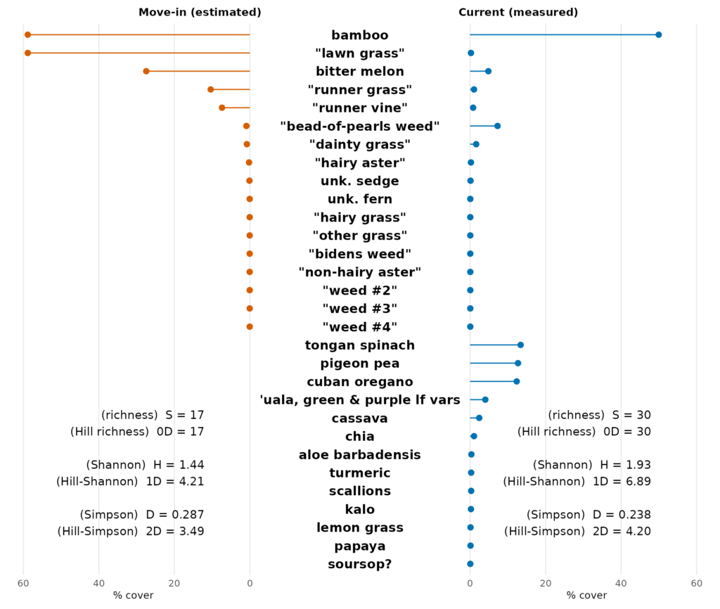
As before, we see the % cover for each species from the “move-in” (i.e., pre-gardening) inventory on the left and the same for the recent inventory on the right. For each inventory, I calculated richness, Shannon index, and Simpson index, which are displayed in sequence with their Hill counterparts. This allows one to quickly compare between traditional and Hill counterparts (i.e., up and down) and between the two inventories (left and right).
So let’s take a look at these numbers. First off: richness. We can see that a simple species count (S) andHill richness (0D) are the same: 17 species at move-in vs. 30 species currently. S and 0D are equivalent. Thus, we can say that richness increased about 1.76x or increased by 13 species.
But it gets more interesting when we look at the Shannon index (H). As I understand it, H is a measure of uncertainty about a species selected randomly from the sample. For example, in a garden dominated by bamboo, one could be fairly certain that a random selection would select bamboo, so the uncertainty would be low. On the other hand, a garden in which all species are present in equal abundance would have a relatively high uncertainty, because a random selection could be one of any number of species. The interpretation gets even more abstract when we’re dealing with relative abundance in terms of proportional cover (as with my dataset) rather than individual counts.
A relatively small Shannon index indicates a relatively low level of diversity and vice versa. This aspect is fairly intuitive. But the units of H are abstract and don’t correspond to anything physical or countable. So, while we can say that my garden is more diverse now (H = 1.93) than it was at move-in (H = 1.44), because of the abstract units of the Shannon index, it’s hard to interpret those numbers in terms of anything tangible.
That’s where Hill diversity makes an improvement. Hill-Shannon diversity (1D) is calculated as: 1D = eH, where e is the constant, Euler’s number (~2.718) and H is the Shannon index. Thus, 1D is just a mathematical transformation of the Shannon index. The result of this transformation is that 1D has a more intuitive unit of measure: number of species. So, comparing Hill-Shannon (1D) values, my garden is more diverse now (1D = 6.89 species) than it was at move-in (1D = 4.21 species).
But what do these values mean exactly? Take the current value, 6.89 species. This means that my garden has the same Hill-Shannon value (1D) as a garden with 6.89 equally abundant species. At move-in, my garden had the same 1D as a garden with only 4.21 equally abundant species. I admit, the concept of fractional species is still a bit abstract. But I can much more easily grasp the concept of species as a unit of measure as opposed to the abstract unit that H uses. And the interpretation of equally abundant is straightforward whether one is using individual counts or proportional cover, which is not the case with H, as I mentioned earlier.
Furthermore, by dividing the two 1D values, I can say that my garden is about 1.64x as diverse now as it was at move-in, or that it has increased in diversity by about 2.68 effective species. That’s easier for me to grasp.
Lastly, let’s take a look at the Simpson index (D). When using individual counts, this is the probability–ranging from 0 to 1–that two randomly selected individuals will be from the same species. In a community dominated by one species (i.e., relatively low diversity), it would be highly likely that two randomly selected individuals would be of the same species, so D would be closer to 1. In contrast, in a community with an even distribution of species (i.e., relatively high diversity), that probability would be low, so D would be closer to 0.
There are some problems with D. First, D is high when diversity is low and vice versa. In my dataset, D was higher at move-in (0.287) than it is currently (0.238), which means that diversity was lower at move-in. Not intuitive. Second, the units of D are not intuitive. The Gini-Simpson index (not calculated for this article) solves the first problem by subtracting D from 1, but the second problem remains.
Hill-Simpson diversity (2D) solves both of these problems. It is calculated as 2D = 1/D, where D is the Simpson index. Thus, 2D increases as diversity increases. And 2D has units of species, the same as 0D, 1D, and all of the other Hill numbers (not covered in this article). And the interpretation is analogous to that of Hill-Shannon diversity. So for example, my garden at move-in had the same Hill-Simpson diversity as a garden with 3.49 equally abundant species whereas currently, that number is 4.20. Thus, plant diversity increased by a factor of 1.20x or about 0.71 effective species.
One thing to point out about Hill numbers is that rare species count less and less towards diversity as we move from richness (0D) to Hill-Shannon (1D) to Hill Simpson (2D). Or we could say that common/dominant species count more and more. For example, the current richness of my garden is 30 species, Hill-Shannon diversity is 6.89, and Hill-Simpson diversity is 4.20. Perhaps yet another way to say this is that the evenness penalty increases as one moves up the Hill number continuum. Thus, when comparing diversity among different communities (in space or in time), the researcher should make a conscious, informed decision about how much to weight rare vs. common species and, as a consequence, which diversity metric to use.
Closing thoughts
In summary, by all five metrics, the plant diversity in my garden is greater now than it was before I started gardening. But there are differences in how the metrics are interpreted. I prefer the Hill numbers, because the units of effective species make them easier to grasp.
As I pointed out, the various Hill numbers differ in how much weight they give to evenness. The most extreme case of species richness (0D) weights all species the same, regardless of relative abundance. In other words, it does not take into account evenness. But the other Hill numbers do.
So what exactly is evenness, and how is it quantified? I plan to explore that question in my next article.
AI RESPONSIBILITY RUBRIC
This rubric shows human vs AI contribution across stages of developing the article. The rubric was generated by AI and reviewed by Taylan, making adjustments as needed.
--------------------
CONCEPT/PLANNING
Human 50% | AI 50%
[==========..........]
Independent study of source literature shaped the article's direction and index selection; collaborative session work refined that into outline structure, interpretive framing, and scope decisions.
--------------------
RESEARCH/VERIFICATION
Human 40% | AI 60%
[========............]
Independent reading of primary and supplementary sources informed the article's factual basis; AI-assisted verification checked citations, caught a logical inconsistency, and supported proofreading.
--------------------
WRITING
Human 80% | AI 20%
[================....]
First draft was written independently and brought to the session in largely polished form, with light AI-assisted editing thereafter.
--------------------
DATA/VISUALIZATION
Human 65% | AI 35%
[=============.......]
Base chart structure originated from AI-generated code in a prior session; the diversity metric calculations and figure extension for this article were done independently in R.
--------------------
IMAGE
Human 90% | AI 10%
[==================..]
Featured image cropping was done independently, with AI input limited to discussing crop options and rationale.
--------------------
EDITING/REFINEMENT
Human 20% | AI 80%
[====................]
AI-assisted fact-checking, logical consistency review, and proofreading pass identified and helped resolve several issues in the draft.
--------------------

AI Tools: Claude Sonnet 5