
Welcome back! This is my fourth article in a mini-series exploring biodiversity, using the plant community in my home garden as an example.
In the first article, I presented the results of a botanical inventory of the garden, using cover proportion as my measure of plant species abundance. In the second article, I compared the recent inventory with an earlier point in time, before I started gardening. And in the third article, I calculated various diversity indices for each of the two time points, doing side-by-side comparisons for illustration.
Now, in the current article, I explore evenness.
What is evenness?
In the context of biodiversity, evenness describes how evenly abundance is distributed among the species of a population. For example, a population in which all species are equally abundant is perfectly even, whereas a population in which the abundance of one species dominates all others is very uneven.
But how does one quantify this evenness?
In a moment, I’ll show the results of evenness calculations for the two time points of my garden. But before I do that, I want to address something I wrote back in the second article.
In that article, I explained that richness (the number of species) and evenness are aspects of diversity. While there is still some truth to this, I recently learned from a 2010 article by Lou Jost titled “The Relation between Evenness and Diversity” that the story is more nuanced.
Namely, richness and evenness are not completely independent of one another. This means that diversity cannot be cleanly split between richness and evenness components. So, while I still find it useful to think of richness and evenness as aspects of diversity, these two aspects are not totally separate things.
As an interesting side note, Jost demonstrates mathematically how diversity and evenness are independent aspects of richness. Conceptually, that’s harder for me to wrap my mind around, and I won’t go into this topic in any more depth in the current article, but I think it is interesting nonetheless. Overall, it’s a pretty math-heavy paper.
How to calculate evenness
As it turns out from my reading of Jost, there are many ways that evenness can be calculated. This is similar to the situation I presented in the previous article in which there are many ways to calculate diversity. (Another interesting side note: there is a lot of overlap in the math presented in the Jost paper between the fields of ecology and economics!)
I’ll cover two types of evenness measures in this article: absolute and relative.
Of the two, the one I find easier to understand–both conceptually and mathematically–is absolute evenness. In reality, there are many absolute evenness metrics. I’ll focus on just one: an evenness factor (EF) derived from Hill-Shannon diversity (1D) and species richness (S). EF is calculated as follows:
EF = 1D / S
As a result, the range of possible values of EF is [1/S, 1]. In other words, the range varies based on the value of S (richness).
The second type is relative evenness, which I find a bit trickier to interpret. This metric, called Pielou’s J, is also derived from Hill-Shannon diversity (1D) and species richness (S):
J = ln(1D) / ln(S)
Unlike EF, the range of possible values of J is always [0, 1], regardless of the value of S. Apparently, this property of J is what makes it more appropriate for making certain comparisons among populations. I’ll admit that I don’t yet understand relative evenness well enough to interpret and explain such comparisons.
Revisiting the garden inventory data
Below are two side-by-side lollipop charts, comparing plant species abundances in the garden plot at move-in (i.e., before I started gardening) and in a more recent, “current” state. For anyone who’s been following along, this graph should look familiar. The only difference from the previous version is in the metrics printed near the bottom of the charts.
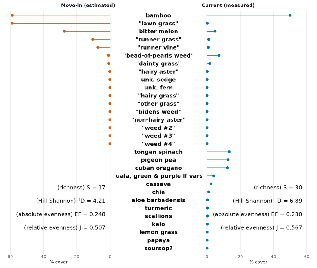
First, let’s look at what’s happening with absolute evenness (EF). Remember, this is derived by dividing 1D by S, both of which have “number of species” as the unit of measure. Recall from the previous article that 1D is an “effective number of species”. This means that my garden at move-in had the same diversity as a perfectly even plant community with 4.21 plant species; it’s “behaving” like a community with about 4 evenly distributed species.
The maximum value that 1D could possibly take is 17, which is equivalent to species richness (S). Thus, EF is the proportion of the actual number of effective species to the maximum possible value of effective species.
EF for the move-in inventory is 0.248, or roughly one-quarter. One way to interpret this is that the diversity of my garden at that time point is about one-quarter of what it could be if all species were equally abundant. Or, as Claude has explained to me, about one-quarter of the species were common.
Compare that to the “current” time point in which EF is 0.230. This is only slightly lower than the move-in time point, which means that in absolute terms the plant community in my garden became slightly less even (or more uneven) in terms of proportional cover as a result of my gardening practices. But still, the absolute evenness is roughly one-quarter, meaning that the diversity of my garden in its “current” state is about one-quarter of what it could be if all 30 species were equally abundant.
Relative evenness (J) tells a story that is similar in one way and different in another. While I understand the math behind it, I still have a hard time understanding the interpretation well enough to explain in my own words, so I’ll simply point out some numerical observations. J is still similar between the two time points (0.507 vs. 0.567). But unlike with EF (absolute evenness), J actually increased as a result of my gardening practices.
Closing thoughts
Back in my second article in this mini-series, when I was visually assessing the inventory data, I wrote that I wasn’t seeing a clear difference in evenness between the two time points. Looking back at my line of reasoning, I can see that what I was visually assessing was absolute evenness. So it’s not surprising to me that it turned out to be very similar between the two time points. And, although I’m not yet confident enough to explain why or what it means, relative evenness didn’t change drastically either.
You may have noticed that I’ve been referring to the most recent inventory as representing the “current” state of my garden. In general, my use of double quotes is an acknowledgment that the plant community is always changing. But also, my garden has very recently undergone more drastic changes: I’ve removed a large portion of the plants that were there and will be removing more. It could be an interesting third time point for comparison.
But that’s a story for another article!
AI RESPONSIBILITY RUBRIC
This rubric shows human vs AI contribution across stages of developing the article. The rubric was generated by AI and reviewed by Taylan, making adjustments as needed.
--------------------
CONCEPT/PLANNING
Human 50% | AI 50%
[==========..........]
Takeaway, scope, and section structure were worked out collaboratively through iterative discussion.
--------------------
RESEARCH/VERIFICATION
Human 45% | AI 55%
[=========...........]
Primary source (Jost 2010) was read independently by the author; AI assisted with explaining and clarifying technical content, and performed a logical/fact-check pass against the source material.
--------------------
WRITING
Human 85% | AI 15%
[=================...]
Draft prose was authored independently; AI contributed to earlier conceptual framing that shaped some phrasing.
--------------------
DATA/VISUALIZATION
Human 60% | AI 40%
[============........]
Figure built on the author's own prior R script and calculations; AI assisted with a formatting fix for chart annotation text.
--------------------
IMAGE
Human 90% | AI 10%
[==================..]
Featured image independently sourced and selected by the author from Jost 2010 (open-access); AI assisted with diagnosing a recurring featured-image cropping issue and generating a correctly-padded version for the theme's aspect ratio.
--------------------
EDITING/REFINEMENT
Human 20% | AI 80%
[====................]
Author made light structural edits prior to review; AI performed line editing, proofreading, and consistency checks.
--------------------

AI Tools: Claude Sonnet 5